Showing posts with label ken. Show all posts

Sunday, April 30, 2017

*** sqlite 3 rls.db , result table

sqlite3 on rls.db

see https://www.tutorialspoint.com/sqlite/


.open rls.db
.databases
.tables
.separator ::
.headers on
.mode column
select distinct experiment from result_experiment limit 20;
.indices
.indices set
.width 5
select * from result  limit 1;

/* The following select can take rls and its reference rls */
select experiments,set_name,set_strain,set_background,set_genotype,
 set_lifespan_mean,ref_genotype,ref_lifespan_mean
 from result  limit 2;

CREATE TEMPORARY TABLE my_RLS_out AS
SELECT experiments,set_name,set_strain,set_background,set_genotype,
 set_lifespan_mean,ref_genotype,ref_lifespan_mean
 FROM result; 

DROP TABLE my_RLS_out;
CREATE TEMPORARY TABLE my_RLS_out AS
SELECT experiments,set_name,set_strain,set_background,set_genotype,
 set_lifespan_mean,ref_genotype,ref_lifespan_mean, ranksum_p
 FROM result
 WHERE ranksum_p < 0.05
 ;

select * from my_RLS_out limit 5;    

select distinct set_genotype from my_RLS_out; 


sqlite> .indices result
result_percent_change
result_pooled_by
result_ranksum_p
result_ref_background
result_ref_genotype
result_ref_locus_tag
result_ref_mating_type
result_ref_media
result_ref_name
result_ref_strain
result_ref_temperature
result_set_background
result_set_genotype
result_set_lifespan_mean
result_set_locus_tag
result_set_mating_type
result_set_media
result_set_name
result_set_strain

result_set_temperature

#output result table into csv
sqlite> .headers on
sqlite> .mode csv
sqlite> .output qintest.csv
sqlite> select * from result;
sqlite> .quit
emc313b02:data hqin$ ll
total 146712
-rw-r--r--  1 hqin  staff   8.5M Apr 30 23:31 qintest.csv
lrwxr-xr-x  1 hqin  staff    15B Apr 30 20:07 rls.db -> rls_20160802.db
-rw-------  1 hqin  staff   8.3M Aug  9  2016 rls_2016-08-02.csv
-rw-------  1 hqin  staff    55M Aug  9  2016 rls_20160802.db
emc313b02:data hqin$ less qintest.csv 
emc313b02:data hqin$ open qintest.csv 

emc313b02:data hqin$ 


Note
Based on
http://stackoverflow.com/questions/18671/quick-easy-way-to-migrate-sqlite3-to-mysql
Sqlite database is not easily convertable to mysql database. 

Sunday, January 11, 2015

Calculate RLS for single-gene mutant

I could modify _Survival Analysis Gomp Weib_20140705qin.R to do this. However, I apparently finished this work in "_explore.20140705.R". In this script, I also used SceORF_name.csv to pick up the single-gene mutant.  I did exactly the same thing half a year later.

"ken-RLS-byORF20150111.csv" is the output file. 

Modified "_explore.20140705.R".
rm(list=ls())
setwd("~/projects/0.network.aging.prj/9.ken")

list.files()

tb = read.csv('conditionsWeibRedo_qin.csv') 
tb$genotypeOri = tb$genotype #change 20150111
tb$genotype = toupper( as.character(tb$genotype)) 
tb$media = as.character(tb$media)
str(tb)

tb[grep("ctf", tb$genotype, ignore.case=T), ]


tb2 = read.csv("SceORF_name.csv", header=F, colClass=c("character", "character"))
names(tb2) = c('ORF','name')
length(unique(tb$genotype))

table( tb$genotype %in% tb2$name )
table( tb2$name %in% tb$genotype )

tb$flag = tb$genotype %in% tb2$name
sub = tb[tb$flag, ]
sub$ORF = tb2$ORF[match(sub$genotype, tb2$name)]

length(unique(sub$genotype))
x = table(sub$media)
x[grep("YPD",names(x))]
tb$media[grep("% D", tb$media, ignore.case=T)]

write.csv(sub, "ken-RLS-byORF20150111.csv", row.names=F, quote=F)

x = sub[sub$n>30, ]
hist(log10(x$n)/log10(3))
summary(sub)
tb[tb$n>1000,]


done, pool single gene mutant data from rls.csv

I studied ken's old codes, my old codes, and wrote "_export_rls20150111.R".

On 20150111, I found out that I did the work in "_explore.20140705.R".

Export single-gene RLS

File _export_rls20150111.R exports genotype that contains single-element 


After running, I got 4842 files. Very impressive.

~/0.network.aging.prj/ken/rls_csv_single_element
Byte:rls_csv_single_element hqin$ ls | wc -l
    4842


File _export_rls20150111.R 
# Jan 11, 2015 H Qin. 
# I want to export single-gene mutant RLS at 30C and YPD for MATalpha
# based on _export_rls20140709.R
# export rls to individual files. I need them for nrmca fittings. 

#####################################################################################################
#################install and declare needed packaqes for survival analysis
rm(list=ls())

#require('survival')
#library('KMsurv')
library('data.table')
library('RSQLite')
#library('flexsurv')
#library('muhaz')

#########################################################################################################
#########################################################################################################

#####################Declare names of files and folders. Move working directory to desired folder. Establish connection to database
#folderLinearHazard = '//udrive.uw.edu/udrive/Kaeberlein Lab/RLS Survival Analysis 2/Linear Hazard'
Folder = "~/projects/0.network.aging.prj/9.ken"
File = 'rls.db'
setwd(Folder)
drv <- SQLite()
con <- dbConnect(drv, dbname = File)

##########################################################################################################
##########################################################################################################

######################Create a complete table of conditions that have data in the RLS database. 
######################(Each row in this table will be a unique combination of genotype, mating type, media, and temperature

###get unique conditions from "set" columns (experimental treatments/mutations)
conditions1 = dbGetQuery(con, "
  SELECT DISTINCT set_genotype as genotype, set_mating_type as mat, set_media as media, set_temperature as temp
  FROM result
  WHERE pooled_by = 'file'
  ")
### rows in the result table of the database are not mutually exclusive. In some rows, data has sometimes been pooled by genotype, background strain, etc.   

###get unique conditions from "reference" columns (these columns are the control conditions/lifespan results for each row of experimental lifespan results. Rows are not mutually exclusive (1 control to many experimental conditions)
conditions2 = dbGetQuery(con, "
  SELECT DISTINCT ref_genotype as genotype, ref_mating_type as mat, ref_media as media, ref_temperature as temp
  FROM result 
  WHERE pooled_by = 'file'
  ")

####combine and take unique conditions from these two
conditions = rbind(conditions1, conditions2)
conditions = unique(conditions)
conditions = conditions[complete.cases(conditions),]
row.names(conditions) = NULL ###renumber the rows. important because future processes will refer to a unique condition by its row number in this table
controlConditions = conditions[conditions$genotype %in% c('BY4741', 'BY4742', 'BY4743'),] ###create a table of conditions that have WT genotypes

head(conditions)
table(conditions$media)

### 2015 Jan 11
### Qin will limit conditions to single-gene, 30C, YPD, MATalpha
conditions = conditions[!is.na(conditions$genotype), ]
conditions = conditions[ conditions$media=='YPD' & conditions$temp==30 & conditions$mat=='MATalpha', ]
conditions$single_element_flag = 0
for( i in 1:length(conditions[,1])) { 
 elements = unlist( strsplit(  conditions$genotype[i], '\\s+',))
 conditions$single_element_flag[i]= length( elements )
}
summary(conditions)
conditions= conditions[conditions$single_element_flag==1 , ]

###Add columns to the conditions data frame. These columns will be filled in by their respective variable: ie. gompertz shape/rate of the lifespan data associated with a given conditions (genotype, mating type, media, temp)
conditions$n = apply(conditions, 1, function(row) 0)
conditions$avgLS = apply(conditions, 1, function(row) 0)
conditions$StddevLS = apply(conditions, 1, function(row) 0)
conditions$medianLS = apply(conditions, 1, function(row) 0)
conditions$gompShape = apply(conditions, 1, function(row) 0)
conditions$gompRate = apply(conditions, 1, function(row) 0)
conditions$gompLogLik = apply(conditions, 1, function(row) 0)
conditions$gompAIC = apply(conditions, 1, function(row) 0)
conditions$weibShape = apply(conditions, 1, function(row) 0)
conditions$weibScale = apply(conditions, 1, function(row) 0)
conditions$weibLogLik = apply(conditions, 1, function(row) 0)
conditions$weibAIC = apply(conditions, 1, function(row) 0)

#############################################################################################################
#############################################################################################################

#########################################Loop through the conditions to get lifespan data 
# r =1

for (r in 1:length(conditions$genotype)) {
  genotypeTemp = conditions$genotype[r]
  mediaTemp = conditions$media[r]
  temperatureTemp = conditions$temp[r]
  matTemp = conditions$mat[r]
  
  conditionName = apply(conditions[r,1:4], 1, paste, collapse=" ") #### create a string to name a possible output file
  conditionName = gsub("[[:punct:]]", "", conditionName) #### remove special characters from the name (ie. quotations marks, slashes, etc.)

  genotypeTemp = gsub("'", "''", genotypeTemp)
  genotypeTemp = gsub('"', '""', genotypeTemp)
  
  ##### Query the database to take data (including lifespan data) from every mutually exclusive row (pooled by file, not genotype, not background, etc). 
  ##### There will often be multiple rows (representing different experiments) for each unique condition. This analysis pools lifespan data from multiple experiments if the conditions are all the same
  queryStatementSet = paste(
    "SELECT * ",
    "FROM result ",
    "WHERE pooled_by = 'file' AND set_genotype = '", genotypeTemp, "' AND set_mating_type = '", matTemp, "' AND set_media = '", mediaTemp, "' AND set_temperature = '", temperatureTemp, "'", 
    sep = ""
  )
  
  queryStatementRef = paste( ### both the reference and set columns will be searched for matching conditions
    "SELECT * ",
    "FROM result ",
    "WHERE pooled_by = 'file' AND ref_genotype = '", genotypeTemp, "' AND ref_mating_type = '", matTemp, "' AND ref_media = '", mediaTemp, "' AND ref_temperature = '", temperatureTemp, "'", 
    sep = ""
  )
  
  dataListSet = dbGetQuery(con, queryStatementSet)
  dataListRef = dbGetQuery(con, queryStatementRef)
  lifespansChar = unique(c(dataListSet$set_lifespans, dataListRef$ref_lifespans)) ### combine lifespan values for a given condition into a single data structure. (problems of having non-mutually exclusive rows in the ref_lifespans column are overcome by only taking unique groups of lifespans. The assumption is that no two experiments produced identical lifespan curvs)
  
  ##### Database codes the lifespan data for each experiment as a string. So, lifespanChar is a vector of strings
  ##### Convert lifespanChar into a single vector of integers lifespansTemp
  lifespansTemp = c()
  if (length(lifespansChar) > 0) {
    for (s in 1:length(lifespansChar)) {
      lifespansNum = as.numeric(unlist(strsplit(lifespansChar[s], ",")))
      lifespansNum = lifespansNum[!is.na(lifespansNum)]
      if (length(lifespansNum) > 0) {
        lifespansTemp = c(lifespansTemp, lifespansNum)
      } 
    }
  }
  
  if (length(lifespansTemp) > 3 ) {
    require(stringr)
    conditions$media[r] = str_replace( conditions$media[r], "\\/", "")
    conditions$media[r] = str_replace( conditions$media[r], "\\/", "")
    conditions$media[r] = str_replace( conditions$media[r], "\\+", "")
    conditions$genotype[r] = str_replace( conditions$genotype[r], "\\/", "-")
    conditions$genotype[r] = str_replace( conditions$genotype[r], "\\/", "-")
    conditions$genotype[r] = str_replace( conditions$genotype[r], "\\/", "-")
    conditions$genotype[r] = str_replace( conditions$genotype[r], "\\/", "-")
    conditions$n[r] = length(lifespansTemp)   #### record number of individuals 
    filename = paste( 'rls_csv_single_element/',conditions$genotype[r], '_', conditions$mat[r],'_temp', conditions$temp[r],
                      '_media_', conditions$media[r], '_n',conditions$n[r], '.csv',sep='')
    out = data.frame(lifespansTemp)
    names(out) = c("rls")
      write.csv(out, filename, quote=F, row.names=F)
  }
  
}#outer loop  


Reorganize the files in rls_csv with n>30


Reorganize the files in rls_csv with n>30

~/0.network.aging.prj/ken/rls_csv.n.gr30/
total 0
drwxr-xr-x   943 hqin  staff    31K Jan 11 19:20 MATa
drwxr-xr-x  2282 hqin  staff    76K Jan 11 19:21 MATalpha
drwxr-xr-x   269 hqin  staff   8.9K Jan 11 19:21 diploid

drwxr-xr-x     4 hqin  staff   136B Jan 11 19:22 unknown

I need to pick out the single gene mutants. 


564 RLS data from Kaeberlein 05 Science

The 2005 564 RLS data were provided both in Kaeberlein05Science and Managbanag08PlosOne.

In K05, genes were separated into LL, NLL, and SL.  LL null mutants extend RLS >=30%. Putatively, LL RLS <= 20, and LL RLS >=36.  Experiments were repeated until classification can be established. In K05, LL strains can extend RLS with Wilcoxon rank-sum test p-value <0.1, and NSE mutants are those with RLS longer than WT but with p-value >0.1


Byte:Kaeberlein05Science hqin$ cat confirmed.LL.txt 
YNR051C BRE5
YDR110W FOB1 
YOR136W IDH2
YBR267W REI1
YLR371W ROM2 
YDL075W RPL31A 
YLR448W RPL6B
YJR066W TOR1
YNL229C URE2
YBR238C 
YBR255W 
YBR266C

There are 13 LL genes in this list, too few for svm training. It seems that I expanded this list using the ratio of mutant/wt RLS. K05 initially identified 44 putative LL, but only 13 were significant.

Q: How are these categories hold in He14 classification? Why did He14 did not use Kaeberlein05 data?

I need to compare Kaberlein05 with He14 classifications.


Sunday, January 4, 2015

parse single mutant rows in rls.csv in R

Parse rls.csv in R to pick single-gene mutant rows.

bug on multiple entries of NAME-to-ORF mapping. This seems to be 8 bugs in file "SceORF_name.csv".


It seems that probably four ORFs share the same gene NAMES, probably due to merged annotations.  I need to revisit this annotation problem. 


The for-loop parsing of 50681 rows took about 2.5 hours on Byte, an apple laptop. 


Impressive. There 4101 single-gene RLS measures?! Visual check of ORF seems to confirm this. These covered almost all the essential genes. 

write.csv(tb,"rls_20150103.csv", quote=T, row.names=F )
#Visual check in Excel. All fields seem correct. 

R script is: "_find_LL_20150104.R", pwd ~/0.network.aging.prj/9.ken/

########  "_find_LL_20150104.R"
setwd("~/projects/0.network.aging.prj/9.ken")
rm(list=ls())

list.files(pattern='csv')

#get sce ORF and names
tb.sce = read.csv("SceORF_name.csv",header=F, colClasses = c(rep('character',2)))
str(tb.sce)
names(tb.sce)= c('ORF','NAME')
set_sce_names = unique(c(tb.sce$ORF, tb.sce$NAME)) #this is the dictionary


tb = read.csv("rls.csv", colClasses=c("integer", rep("character",8),
                                      rep("numeric",5), rep("character",8),
                                      rep("numeric",5),'character',
                                      rep('numeric',3), 'character')
              )
str(tb)

tb$setRLS_vs_ref_RLS = tb$set_lifespan_mean / tb$ref_lifespan_mean
hist(tb$setRLS_vs_ref_RLS, br = 30)
summary(tb$ranksum_p)
tb$LL = ifelse( tb$ranksum_p <0.05 & tb$setRLS_vs_ref_RLS>1, 'LL', 'NLL' )
table(tb$LL)

sort( unique(toupper(tb$set_genotype[tb$LL=='LL'])) ) 

# need to pick up single-gene mutants from tb$set_genotype 
tb$ORF = NA; tb$NAME = NA; tb$single_gene_flag = 0;
for( i in 1:length(tb[,1])) { 
#for( i in 1:100) {
  print (paste("i=",i))
  elements = strsplit(  tb$set_genotype[i], '\\s+',)
  current_name = toupper(elements[[1]][1])
  if (( current_name %in% set_sce_names) & (length(elements)==1 )){
    if (current_name %in% tb.sce$NAME) {
      tb$ORF[i] = tb.sce$ORF[tb.sce$NAME == current_name]
      tb$NAME[i] = current_name;
      tb$single_gene_flag[i] = 1;
    } else if (current_name %in% tb.sce$ORF ) {
      tb$NAME[i] = tb.sce$NAME[tb.sce$ORF == current_name]
      tb$ORF[i] = current_name;
      tb$single_gene_flag[i] = 1;  
    } else {
      print ("Excuse me. NAME or ORF seems weird at line 42. tb$single_gene_flag set to -1.")
      tb$single_gene_flag[i] = -1;
    }     
  }
} #run from 12:38- about 3pm. 

save.image("_20150104.RData")
table( tb$single_gene_flag)
length( unique(tb$ORF[tb$single_gene_flag == 1]) )

write.csv(tb,"rls_20150104.csv", quote=T, row.names=F )
######## end of  "_find_LL_20150104.R"


Saturday, January 3, 2015

parse single mutant rows from rls.csv in python

I wrote a python 2.7 script to pick single-gene mutant from set_genotype and output into a new csv file for R analysis.

I used the 'SceORF_name.csv' to generate a dictionary first.
(Python picked up two rows MF(ALPHA)1 and MF(ALPHA)2 without comma. I nano fixed this.)

I then pick set_genotype with a single element that exist in SceORF_name. For R analysis, I output ORF and NAME.

Trouble: 'rls.csv' stores quoted raw lifespan with commas. These quotes disappeared after python parsing and cause confusion in csv format.
Option1: output in tab format. ==> Still have problems.
Option 2: add quotes back to set_lifespans. ==> Seems to works fine in Excel, but not in R. 
(There are 29839 rows in Excel, but R read 35K rows). 
Option 3: convert csv to xlsx and read.xlsx(). ==> not enough memory to run read.xlsx()

11:43pm. Through converting xlsx to csv, I found many extra empty columns in the file. I copy-pasted the 34 columns into a new csv file. This time, load into R show 29838 observations. This is correct.
File 'single_gene_mutants_frm_filerlscsv_20150103.csv' is the output file. (wrong format!)


Python script is parse_rlscsv_20150103.py

20150104: checking in R found wrong values in many columns. Perhaps the best way to parse 'rls.csv' in R directly.

Option 4: remove the set_lifepans


#####################parse_rlscsv_20150103.py
import StringIO
import csv
import re

# parse ORF name pairs
FL1 = open('SceORF_name.csv', 'rb')
Dic = {} # dictionary
reader1 = csv.reader(FL1, dialect='excel', delimiter=',')
for row in reader1:
ORF = row[0]
NAME = row[1]
if ( not ( ORF in Dic.keys() ) ):
Dic[ORF] = ORF
Dic[NAME] = ORF  


outfile = open( 'single_gene_mutants_frm_filerlscsv_20150103.csv', 'w')
header="ORF,NAME,id,experiments,set_name,set_strain,set_background,set_mating_type,set_locus_tag,set_genotype,set_media,set_temperature,set_lifespan_start_count,set_lifespan_count,set_lifespan_mean,set_lifespan_stdev,set_lifespans,ref_name,ref_strain,ref_background,ref_mating_type,ref_locus_tag,ref_genotype,ref_media,ref_temperature,ref_lifespan_start_count,ref_lifespan_count,ref_lifespan_mean,ref_lifespan_stdev,ref_lifespans,percent_change,ranksum_u,ranksum_p,pooled_by\n"
#header = header.replace(',', '\t')
outfile.write(header)

csvfile = open('rls.csv','rb')
reader = csv.reader(csvfile, dialect='excel', delimiter=',')

for row in reader:
elements = re.split('\s+', row[7] )
current_name = elements[0].upper()
if (len(elements) == 1) & (current_name in Dic.keys()):
row[14] = "\"" + row[14] + "\""
row[27] = "\"" + row[27] + "\""
#outfile.write( Dic[current_name]+'\t'+current_name + '\t'+'\t'.join(row)+ '\n')
outfile.write( Dic[current_name]+','+current_name + ','+','.join(row)+ '\n')

outfile.close()

#####################end of parse_rlscsv_20150103.py


compare result table and rls.csv

rls.csv contains 50681 observations of 32 variables

in sqlite3 on rls.db
select max(id) from result
/* this is 50689 */

So, result table in rls.db contains similar entries in rls.csv.

_find_LL_20150103.r

# _find_LL_20150103.r

rm(list=ls())
tb = read.csv("rls.csv", colClasses=c("integer", rep("character",8),
                                      rep("numeric",5), rep("character",8),
                                      rep("numeric",5),'character',
                                      rep('numeric',3), 'character')
              )
str(tb)

tb$setRLS_vs_ref_RLS = tb$set_lifespan_mean / tb$ref_lifespan_mean
hist(tb$setRLS_vs_ref_RLS, br = 30)
summary(tb$ranksum_p)
tb$LL = ifelse( tb$ranksum_p <0.05 & tb$setRLS_vs_ref_RLS>1, 'LL', 'NLL' )
table(tb$LL)

sort( unique(toupper(tb$set_genotype[tb$LL=='LL'])) )

# need to pick up single-gene mutants from tb$set_genotype
tb$single_gene_mutant = 1;
tb$single_gene_mutant[grep( "[\\s|\\/]+", tb$set_genotype)] = 2
table(tb$single_gene_mutant)
summary(tb$single_gene_mutant)

tb.s = tb[tb$single_gene_mutant == 1, ]
#tb.s contains only single element
sort( unique(toupper(tb.s$set_genotype[tb.s$LL=='LL'])) )
head(tb.s)


Saturday, December 27, 2014

SQLite3 code on rls.db

file 'test_rls.sql'

.open rls.db
.databases
.tables
.separator ::
.headers on
.mode column
select distinct experiment from result_experiment limit 20;
.indices
.indices set
.width 5
select * from result  limit 1;

/* The following select can take rls and its reference rls */
select experiments,set_name,set_strain,set_background,set_genotype,
 set_lifespan_mean,ref_genotype,ref_lifespan_mean
 from result  limit 2;


/* The fields of set_name and set_genotype sometimes provide the ORF-name pair, but there are many exceptions. */


SQLite 3, osX, byte, rls.db

Reference: http://www.sqlite.org/cli.html


#I want to install SQLite to load 'rls.db'. 

$ sudo port install sqlite3
#OK

#how to load 'rls.db' ?
$ sqlite3 
SQLite version 3.8.7.4 2014-12-09 01:34:36
Enter ".help" for usage hints.
Connected to a transient in-memory database.
Use ".open FILENAME" to reopen on a persistent database.
sqlite> .open rls.db
sqlite> .databases
seq  name             file                                                      
---  ---------------  ----------------------------------------------------------
0    main             /Users/hqin/projects/0.network.aging.prj/4.svm/rls.db     
sqlite> .tables
build_log           genotype_pubmed_id  result_experiment   set               
cross_mating_type   meta                result_ref          yeast_strain      
cross_media         result              result_set 

sqlite> .indices
build_log_filename
cross_mating_type_background
cross_mating_type_genotype
cross_mating_type_locus_tag
cross_mating_type_media
cross_mating_type_temperature
cross_media_background
cross_media_genotype
cross_media_locus_tag
cross_media_mating_type
cross_media_temperature
genotype_pubmed_id_genotype
genotype_pubmed_id_pubmed_id
meta_name
result_experiment_experiment
result_experiment_result_id
result_percent_change
result_pooled_by
result_ranksum_p
result_ref_background
result_ref_genotype
result_ref_locus_tag
result_ref_mating_type
result_ref_media
result_ref_name
result_ref_result_id
result_ref_set_id
result_ref_strain
result_ref_temperature
result_set_background
result_set_genotype
result_set_lifespan_mean
result_set_locus_tag
result_set_mating_type
result_set_media
result_set_name
result_set_result_id
result_set_set_id
result_set_strain
result_set_temperature
set_experiment
set_media
set_name
set_strain
set_temperature
yeast_strain_background
yeast_strain_genotype_short
yeast_strain_genotype_unique
yeast_strain_mating_type
yeast_strain_name
yeast_strain_owner

sqlite> select distinct experiment from result_experiment limit 20;
experiment
1
100
101
102_plate115
103
104
105
106_plate116
107
108_plate117
... 

sqlite> .separator :::
sqlite> select * from result limit 2;
id:::experiments:::set_name:::set_strain:::set_background:::set_mating_type:::set_locus_tag:::set_genotype:::set_media:::set_temperature:::set_lifespan_start_count:::set_lifespan_count:::set_lifespan_mean:::set_lifespan_stdev:::set_lifespans:::ref_name:::ref_strain:::ref_background:::ref_mating_type:::ref_locus_tag:::ref_genotype:::ref_media:::ref_temperature:::ref_lifespan_start_count:::ref_lifespan_count:::ref_lifespan_mean:::ref_lifespan_stdev:::ref_lifespans:::percent_change:::ranksum_u:::ranksum_p:::pooled_by
1:::127:::BY4741:::KK19:::BY4741:::MATa::::::BY4741:::YPD:::30.0:::20:::20:::30.3:::7.526095:::23,26,34,31,22,37,26,39,22,36,38,24,36,40,26,38,38,17,34,19:::BY4742:::DH502:::BY4742:::MATalpha::::::BY4742:::YPD:::30.0:::40:::40:::29.625:::8.279377:::36,26,15,28,16,44,40,28,25,32,24,29,39,37,30,31,14,17,29,28,44,27,38,29,26,39,38,32,34,33,32,38,16,28,31,11,20,39,30,32:::2.278481:::409.0:::0.8916505557143:::file
2:::127:::ymr226c:::DC:4G4:::BY4741:::MATa::::::tma29:::YPD:::30.0:::20:::20:::27.1:::11.702:::24,11,37,32,41,38,12,11,31,23,39,36,22,19,28,36,24,49,24,5:::BY4741:::KK19:::BY4741:::MATa::::::BY4741:::YPD:::30.0:::20:::20:::30.3:::7.526095:::23,26,34,31,22,37,26,39,22,36,38,24,36,40,26,38,38,17,34,19:::-10.56106:::169.5:::0.4163969339623:::file
#Notes, field 'experiments' in 'result' maybe used to find the in-experiment wildtype controls. 
# Ken once suggested that "pooled by" column?? file, genotype, mixed
# set lifespan
# ref lifespan


select experiments,set_name,set_strain,set_background,set_genotype,
 set_lifespan_mean,ref_genotype,ref_lifespan_mean

 from result  limit 2;


Thursday, July 31, 2014

ken rls

"pooled by" column?? file, genotype, mixed

set lifespan
ref lifespan

Wednesday, July 9, 2014

extract rls in csv format from rls.db


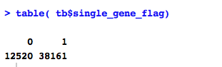
548 rls*.csv files are extracted with sample size > 100.


file "_export_rls20140709.r"

#export rls to individual files. I need them for nrmca fittings.

#####################################################################################################
#################install and declare needed packaqes for survival analysis
rm(list=ls())


#require('survival')
#library('KMsurv')
library('data.table')
library('RSQLite')
#library('flexsurv')
#library('muhaz')

#########################################################################################################
#########################################################################################################

#####################Declare names of files and folders. Move working directory to desired folder. Establish connection to database
#folderLinearHazard = '//udrive.uw.edu/udrive/Kaeberlein Lab/RLS Survival Analysis 2/Linear Hazard'
Folder = "~/projects/0.network.aging.prj/9.ken"
File = 'rls.db'
setwd(Folder)
drv <- SQLite()
con <- dbConnect(drv, dbname = File)

##########################################################################################################
##########################################################################################################

######################Create a complete table of conditions that have data in the RLS database.
######################(Each row in this table will be a unique combination of genotype, mating type, media, and temperature

###get unique conditions from "set" columns (experimental treatments/mutations)
conditions1 = dbGetQuery(con, "
  SELECT DISTINCT set_genotype as genotype, set_mating_type as mat, set_media as media, set_temperature as temp
  FROM result
  WHERE pooled_by = 'file'
  ")
### rows in the result table of the database are not mutually exclusive. In some rows, data has sometimes been pooled by genotype, background strain, etc.

###get unique conditions from "reference" columns (these columns are the control conditions/lifespan results for each row of experimental lifespan results. Rows are not mutually exclusive (1 control to many experimental conditions)
conditions2 = dbGetQuery(con, "
  SELECT DISTINCT ref_genotype as genotype, ref_mating_type as mat, ref_media as media, ref_temperature as temp
  FROM result
  WHERE pooled_by = 'file'
  ")

####combine and take unique conditions from these two
conditions = rbind(conditions1, conditions2)
conditions = unique(conditions)
conditions = conditions[complete.cases(conditions),]
row.names(conditions) = NULL ###renumber the rows. important because future processes will refer to a unique condition by its row number in this table
controlConditions = conditions[conditions$genotype %in% c('BY4741', 'BY4742', 'BY4743'),] ###create a table of conditions that have WT genotypes

###Add columns to the conditions data frame. These columns will be filled in by their respective variable: ie. gompertz shape/rate of the lifespan data associated with a given conditions (genotype, mating type, media, temp)
conditions$n = apply(conditions, 1, function(row) 0)
conditions$avgLS = apply(conditions, 1, function(row) 0)
conditions$StddevLS = apply(conditions, 1, function(row) 0)
conditions$medianLS = apply(conditions, 1, function(row) 0)
conditions$gompShape = apply(conditions, 1, function(row) 0)
conditions$gompRate = apply(conditions, 1, function(row) 0)
conditions$gompLogLik = apply(conditions, 1, function(row) 0)
conditions$gompAIC = apply(conditions, 1, function(row) 0)
conditions$weibShape = apply(conditions, 1, function(row) 0)
conditions$weibScale = apply(conditions, 1, function(row) 0)
conditions$weibLogLik = apply(conditions, 1, function(row) 0)
conditions$weibAIC = apply(conditions, 1, function(row) 0)

#############################################################################################################
#############################################################################################################

#########################################Loop through the conditions to get lifespan data
# r =1

for (r in 1:length(conditions$genotype)) {
  genotypeTemp = conditions$genotype[r]
  mediaTemp = conditions$media[r]
  temperatureTemp = conditions$temp[r]
  matTemp = conditions$mat[r]

  conditionName = apply(conditions[r,1:4], 1, paste, collapse=" ") #### create a string to name a possible output file
  conditionName = gsub("[[:punct:]]", "", conditionName) #### remove special characters from the name (ie. quotations marks, slashes, etc.)

  genotypeTemp = gsub("'", "''", genotypeTemp)
  genotypeTemp = gsub('"', '""', genotypeTemp)

  ##### Query the database to take data (including lifespan data) from every mutually exclusive row (pooled by file, not genotype, not background, etc).
  ##### There will often be multiple rows (representing different experiments) for each unique condition. This analysis pools lifespan data from multiple experiments if the conditions are all the same
  queryStatementSet = paste(
    "SELECT * ",
    "FROM result ",
    "WHERE pooled_by = 'file' AND set_genotype = '", genotypeTemp, "' AND set_mating_type = '", matTemp, "' AND set_media = '", mediaTemp, "' AND set_temperature = '", temperatureTemp, "'",
    sep = ""
  )

  queryStatementRef = paste( ### both the reference and set columns will be searched for matching conditions
    "SELECT * ",
    "FROM result ",
    "WHERE pooled_by = 'file' AND ref_genotype = '", genotypeTemp, "' AND ref_mating_type = '", matTemp, "' AND ref_media = '", mediaTemp, "' AND ref_temperature = '", temperatureTemp, "'",
    sep = ""
  )

  dataListSet = dbGetQuery(con, queryStatementSet)
  dataListRef = dbGetQuery(con, queryStatementRef)
  lifespansChar = unique(c(dataListSet$set_lifespans, dataListRef$ref_lifespans)) ### combine lifespan values for a given condition into a single data structure. (problems of having non-mutually exclusive rows in the ref_lifespans column are overcome by only taking unique groups of lifespans. The assumption is that no two experiments produced identical lifespan curvs)

  ##### Database codes the lifespan data for each experiment as a string. So, lifespanChar is a vector of strings
  ##### Convert lifespanChar into a single vector of integers lifespansTemp
  lifespansTemp = c()
  if (length(lifespansChar) > 0) {
    for (s in 1:length(lifespansChar)) {
      lifespansNum = as.numeric(unlist(strsplit(lifespansChar[s], ",")))
      lifespansNum = lifespansNum[!is.na(lifespansNum)]
      if (length(lifespansNum) > 0) {
        lifespansTemp = c(lifespansTemp, lifespansNum)
      }
    }
  }

  if (length(lifespansTemp) > 100) {
    require(stringr)
    conditions$media[r] = str_replace( conditions$media[r], "\\/", "")
    conditions$genotype[r] = str_replace( conditions$genotype[r], "\\/", "-")
    conditions$n[r] = length(lifespansTemp)   #### record number of individuals
    filename = paste( 'rls_csv/',conditions$genotype[r], '_', conditions$mat[r],'_temp', conditions$temp[r], '_n',conditions$n[r],
                      '_media_', conditions$media[r], '.csv',sep='')
    out = data.frame(lifespansTemp)
    names(out) = c("rls")
      write.csv(out, filename, quote=F, row.names=F)
  }

}#outer loop


Tuesday, July 8, 2014

Select ORF rls

# 9.ken/_explore.20140705

rm(list=ls())
setwd("~/projects/0.network.aging.prj/9.ken")

list.files()

tb = read.csv('conditionsWeibRedo_qin.csv')
tb$genotype = toupper( as.character(tb$genotype))
tb$media = as.character(tb$media)
str(tb)

tb[grep("ctf", tb$genotype, ignore.case=T), ]


tb2 = read.csv("SceORF_name.csv", header=F, colClass=c("character", "character"))
names(tb2) = c('ORF','name')
length(unique(tb$genotype))

table( tb$genotype %in% tb2$name )
table( tb2$name %in% tb$genotype )

tb$flag = tb$genotype %in% tb2$name
sub = tb[tb$flag, ]
sub$ORF = tb2$ORF[match(sub$genotype, tb2$name)]

length(unique(sub$genotype))
x = table(sub$media)
x[grep("YPD",names(x))]
tb$media[grep("% D", tb$media, ignore.case=T)]

write.csv(sub, "ken-RLS-byORF.csv", row.names=F, quote=F)

x = sub[sub$n>30, ]
hist(log10(x$n)/log10(3))
summary(sub)
tb[tb$n>1000,]


Sunday, July 6, 2014

Stddev of 'rls.db'

# ~/9.ken/Survival Analysis Gomp Weib_20140705qin.r

#####################################################################################################
#################install and declare needed packaqes for survival analysis

#install.packages('survival') 
#install.packages('KMsurv')
#install.packages('data.table')
#install.packages('RSQLite')

library('survival')
library('KMsurv')
library('data.table')
library('RSQLite')
library('flexsurv')
library('muhaz')

#########################################################################################################
#########################################################################################################

#####################Declare names of files and folders. Move working directory to desired folder. Establish connection to database
#folderLinearHazard = '//udrive.uw.edu/udrive/Kaeberlein Lab/RLS Survival Analysis 2/Linear Hazard'
Folder = "~/projects/0.network.aging.prj/9.ken"
File = 'rls.db'
setwd(Folder)
drv <- SQLite()
con <- dbConnect(drv, dbname = File)

##########################################################################################################
##########################################################################################################

######################Create a complete table of conditions that have data in the RLS database. 
######################(Each row in this table will be a unique combination of genotype, mating type, media, and temperature

###get unique conditions from "set" columns (experimental treatments/mutations)
conditions1 = dbGetQuery(con, "
  SELECT DISTINCT set_genotype as genotype, set_mating_type as mat, set_media as media, set_temperature as temp
  FROM result
  WHERE pooled_by = 'file'
  ")
### rows in the result table of the database are not mutually exclusive. In some rows, data has sometimes been pooled by genotype, background strain, etc.   

###get unique conditions from "reference" columns (these columns are the control conditions/lifespan results for each row of experimental lifespan results. Rows are not mutually exclusive (1 control to many experimental conditions)
conditions2 = dbGetQuery(con, "
  SELECT DISTINCT ref_genotype as genotype, ref_mating_type as mat, ref_media as media, ref_temperature as temp
  FROM result 
  WHERE pooled_by = 'file'
  ")

####combine and take unique conditions from these two
conditions = rbind(conditions1, conditions2)
conditions = unique(conditions)
conditions = conditions[complete.cases(conditions),]
row.names(conditions) = NULL ###renumber the rows. important because future processes will refer to a unique condition by its row number in this table
controlConditions = conditions[conditions$genotype %in% c('BY4741', 'BY4742', 'BY4743'),] ###create a table of conditions that have WT genotypes

###Add columns to the conditions data frame. These columns will be filled in by their respective variable: ie. gompertz shape/rate of the lifespan data associated with a given conditions (genotype, mating type, media, temp)
conditions$n = apply(conditions, 1, function(row) 0)
conditions$avgLS = apply(conditions, 1, function(row) 0)
conditions$StddevLS = apply(conditions, 1, function(row) 0)
conditions$medianLS = apply(conditions, 1, function(row) 0)
conditions$gompShape = apply(conditions, 1, function(row) 0)
conditions$gompRate = apply(conditions, 1, function(row) 0)
conditions$gompLogLik = apply(conditions, 1, function(row) 0)
conditions$gompAIC = apply(conditions, 1, function(row) 0)
conditions$weibShape = apply(conditions, 1, function(row) 0)
conditions$weibScale = apply(conditions, 1, function(row) 0)
conditions$weibLogLik = apply(conditions, 1, function(row) 0)
conditions$weibAIC = apply(conditions, 1, function(row) 0)

#############################################################################################################
#############################################################################################################

#########################################Loop through the conditions to get lifespan data 
for (r in 1:length(conditions$genotype)) {

  genotypeTemp = conditions$genotype[r]
  mediaTemp = conditions$media[r]
  temperatureTemp = conditions$temp[r]
  matTemp = conditions$mat[r]
  
  conditionName = apply(conditions[r,1:4], 1, paste, collapse=" ") #### create a string to name a possible output file
  conditionName = gsub("[[:punct:]]", "", conditionName) #### remove special characters from the name (ie. quotations marks, slashes, etc.)

  genotypeTemp = gsub("'", "''", genotypeTemp)
  genotypeTemp = gsub('"', '""', genotypeTemp)
  
  ##### Query the database to take data (including lifespan data) from every mutually exclusive row (pooled by file, not genotype, not background, etc). 
  ##### There will often be multiple rows (representing different experiments) for each unique condition. This analysis pools lifespan data from multiple experiments if the conditions are all the same
  queryStatementSet = paste(
    "SELECT * ",
    "FROM result ",
    "WHERE pooled_by = 'file' AND set_genotype = '", genotypeTemp, "' AND set_mating_type = '", matTemp, "' AND set_media = '", mediaTemp, "' AND set_temperature = '", temperatureTemp, "'", 
    sep = ""
  )
  
  queryStatementRef = paste( ### both the reference and set columns will be searched for matching conditions
    "SELECT * ",
    "FROM result ",
    "WHERE pooled_by = 'file' AND ref_genotype = '", genotypeTemp, "' AND ref_mating_type = '", matTemp, "' AND ref_media = '", mediaTemp, "' AND ref_temperature = '", temperatureTemp, "'", 
    sep = ""
  )
  
  dataListSet = dbGetQuery(con, queryStatementSet)
  dataListRef = dbGetQuery(con, queryStatementRef)
  lifespansChar = unique(c(dataListSet$set_lifespans, dataListRef$ref_lifespans)) ### combine lifespan values for a given condition into a single data structure. (problems of having non-mutually exclusive rows in the ref_lifespans column are overcome by only taking unique groups of lifespans. The assumption is that no two experiments produced identical lifespan curvs)
  
  ##### Database codes the lifespan data for each experiment as a string. So, lifespanChar is a vector of strings
  ##### Convert lifespanChar into a single vector of integers lifespansTemp
  lifespansTemp = c()
  if (length(lifespansChar) > 0) {
    for (s in 1:length(lifespansChar)) {
      lifespansNum = as.numeric(unlist(strsplit(lifespansChar[s], ",")))
      lifespansNum = lifespansNum[!is.na(lifespansNum)]
      if (length(lifespansNum) > 0) {
        lifespansTemp = c(lifespansTemp, lifespansNum)
      } 
    }
  }
    
  conditions$n[r] = length(lifespansTemp) #### record number of individuals 
  

  ##### Now that there is a single vector of lifespans for a condition. Do the analysis
  if (length(lifespansTemp) > 4) {
    
    lifespanGomp = flexsurvreg(formula = Surv(lifespansTemp) ~ 1, dist = 'gompertz') ### Use the flexsurvreg package to fit lifespan data to gompertz or weibull distribution
    lifespanWeib = flexsurvreg(formula = Surv(lifespansTemp) ~ 1, dist = 'weibull')  
  
    ### Fill in added columns in the conditions table with data from gompertz and weibull fitting. Columns are named according to respective variables
    conditions$avgLS[r] = mean(lifespansTemp)
    conditions$StddevLS[r] = sd(lifespansTemp)
    conditions$medianLS[r] = median(lifespansTemp)
    conditions$gompShape[r] = lifespanGomp$res[1,1]
    conditions$gompRate[r] = lifespanGomp$res[2,1]
    conditions$gompLogLik[r] = lifespanGomp$loglik
    conditions$gompAIC[r] = lifespanGomp$AIC

    conditions$weibShape[r] = lifespanWeib$res[1,1]
    conditions$weibScale[r] = lifespanWeib$res[2,1]
    conditions$weibLogLik[r] = lifespanWeib$loglik
    conditions$weibAIC[r] = lifespanWeib$AIC    
    }
  

  #### plot survival/hazard/linearized hazard curves. For gompertz fitting data, ln(hazard) should be linear with time (generations). For weibull fitting data ln(hazard) should be linear with ln(generations).
  if(exists('lifespanWeib')) {
    #setwd(folderSurvivalCurves)
    setwd('/tmp/')
    jpeg(paste(conditionName, 'Survival Curve Weibull.jpg'))
    plot(lifespanWeib, xlab = 'generations', ylab = 'S', main = paste(conditionName, 'Survival Curve Weibull'))
    dev.off()
    
    #setwd(folderCumulativeHazard)
    setwd('/tmp/')
    jpeg(paste(conditionName, 'Cumulative Hazard Weibull.jpg'))
    plot(lifespanGomp, type = 'cumhaz', xlab = 'generations', ylab = 'H', main = paste(conditionName, 'Cumulative Hazard Weibull'))
    dev.off()
    
    #setwd(folderLinearHazard)
    setwd('/tmp/')
    jpeg(paste(conditionName, 'Linear Hazard Weibull.jpg'))
    hazard = kphaz.fit(lifespansTemp, rep(1, length(lifespansTemp)))
    plot(log(hazard$time), log(hazard$haz), xlab = 'log(generations)', ylab = 'log(h)', main = paste(conditionName, 'Linear Hazard Weibull')) 
    a = lifespanWeib$res[1,1]
    b = lifespanWeib$res[2,1]
    intercept = log(a/b) - (a-1)*log(b)
    slope = a-1
    abline(intercept, slope)  
    dev.off()
    
    
    rm(lifespanWeib)
    
  }
  
}

setwd(Folder) write.csv(conditions, 'conditionsWeibRedo_qin.csv') ##### output conditions table to a CSV file