protein disorder, robustness

http://biorxiv.org/content/biorxiv/early/2015/11/25/032847.full.pdf

Glucose dose effect on RLS in BY4742, code

File: _BY4742.glucose.dose.20140712.r

#test binomial aging model on glucose dose in BY4742

rm(list=ls());
setwd("~/projects/0.network.aging.prj/0a.network.fitting")
source("lifespan.20140711.r")
require(flexsurv)

pdf("BY4742GlucoseDose-binomial-20140713.pdf", width=10, height=8)
layout(matrix(c(1,2,3,4), 2, 2, byrow = TRUE))

files = list.files(, path='DR', pattern="BY4742")

files = c(
  "BY4742_MATalpha_temp30_media_0.005% D_n299.csv",                
  "BY4742_MATalpha_temp30_media_0.05% D_n4690.csv",                
  "BY4742_MATalpha_temp30_media_0.1% D_n338.csv",                  
  "BY4742_MATalpha_temp30_media_0.5% D_n579.csv",                  
  "BY4742_MATalpha_temp30_media_YPD_n19930.csv"
);

output = data.frame(files);
output$mean = NA; output$stddev = NA; output$CV=NA;
output$R=NA; output$t0=NA; output$n=NA;
output$Rflex = NA; output$Gflex = NA;
output$glucose = c(0.005, 0.05, 0.1, 0.5, 2.0)

#i=1;
for( i in 1:5) {
  filename = paste('DR/', files[i], sep='')
  tb = read.csv(filename)
  summary(tb)
  output$mean[i]=mean(tb$rls)
  output$stddev[i]= sd(tb$rls)
  output$CV[i] = sd(tb$rls) / mean(tb$rls)

  fitGomp = flexsurvreg( formula=Surv(tb$rls) ~ 1, dist='gompertz')
  Rhat = fitGomp$res[2,1]; Ghat = fitGomp$res[1,1]
  output$Rflex[i] = Rhat; output$Gflex[i]=Ghat;

  #G = (n-1) / t0, so t0 = (n-1)/G
  nhat = 3; t0= (nhat-1)/Ghat; t0
  fitBinom = optim ( c(Rhat, t0, nhat),  llh.binomialMortality.single.run , lifespan=tb$rls,
                method="L-BFGS-B", lower=c(1E-10,0.05,1E-1), upper=c(10,100,50) );

  output[i, c("R", "t0", "n")] = fitBinom$par

    #  fitGomp2 = optim ( c(0.005, 0.08),  llh.G.single.run , lifespan=tb$rls,
   #                    method="L-BFGS-B", lower=c(1E-10,1E-2), upper=c(10,10) );

  tb2 = calculate.mortality.rate(tb$rls)
  plot( tb2$s ~ tb2$t, main=filename)
  plot( tb2$mortality.rate ~ tb2$t , main=filename)
  plot( tb2$mortality.rate ~ tb2$t, log='y', main='linear for Gompertz' )
  plot( tb2$mortality.rate ~ tb2$t, log='yx', main='linear for Weibull' )
}#i file loop


plot( output$R ~ output$glucose, type='l' )
plot( output$t0 ~ output$glucose,type='l' )
plot( output$n ~ output$glucose,type='l' )
plot( output$mean ~ output$glucose, type='l')
plot( output$CV ~ output$glucose, type='l' )
plot( output$stddev ~ output$glucose, type='l')
plot( output$Rflex ~ output$glucose, type='l')
plot( output$Gflex ~ output$glucose, type='l')

dev.off()


q('no')
####END of 20140712 #########

robustness 20140709

gompShape batch regression

##############################
# batch regression ~ CV
pTb = 1: length(fit3[1,])
names(pTb) = names(fit3); length(pTb)
pTb[1:15]
#for( j in c(7:50) ) {
for( j in c(7:19, 22:32, 34:538) ) {
  m = lm( fit3[, j] ~ fit3$StddevLS/fit3$avgLS )
  sm = summary(m); sm
  pTb[j] = 1 - pf(sm$fsta[1], sm$fsta[2], sm$fsta[3])
}
pTb[pTb<0.05]
p= pTb[c(22:32, 34:538)]
p[p<0.01]
hist(p, br=20)
source("robust-fdr.R")
ret= robust.fdr(p)
summary(ret$q)
hist(ret$q, br=20)

#There are dozens of factors ~ rls CV, including the PPI degree. 

RLS CV ~ morphology CV (why a negative correlation?)

gompShape ~ morphology CV(positive correlation)?

Todo: I can exclude the small sample size measure to see if p-value can be improved.


RLS CV ~ (-)~ evolutionary measures. High selection pressure -> stronger robustness. 
    Kdata = read.csv( "data/Sce.Spa.KaKs.csv");

20140710note: The gene with small CV and high omega is highly interesting. 

Todo: use log, sqrt() transformation on variables. Remove small sample sized measures, say n<30?

Zhao et al Cell, 2005, navigating chaperone network, hsp90

Hsp90 regulates 10% of the yeast genome, 627 putative hsp90 substrates.

Zhao05Cell used geldanamycin screen 4 times, and found 200 ORFs dependent on Hsp90 for, provided in table S4.

Notable missing 'known(?)' substrates: Ste11, Hap1, Ctf13/Skp1, Rpn components of proteasome.

49 ORF genetically interacts with Hsp90 by SGA and GS.

Stddev of 'rls.db'

# ~/9.ken/Survival Analysis Gomp Weib_20140705qin.r

#####################################################################################################
#################install and declare needed packaqes for survival analysis

#install.packages('survival') 
#install.packages('KMsurv')
#install.packages('data.table')
#install.packages('RSQLite')

library('survival')
library('KMsurv')
library('data.table')
library('RSQLite')
library('flexsurv')
library('muhaz')

#########################################################################################################
#########################################################################################################

#####################Declare names of files and folders. Move working directory to desired folder. Establish connection to database
#folderLinearHazard = '//udrive.uw.edu/udrive/Kaeberlein Lab/RLS Survival Analysis 2/Linear Hazard'
Folder = "~/projects/0.network.aging.prj/9.ken"
File = 'rls.db'
setwd(Folder)
drv <- SQLite()
con <- dbConnect(drv, dbname = File)

##########################################################################################################
##########################################################################################################

######################Create a complete table of conditions that have data in the RLS database. 
######################(Each row in this table will be a unique combination of genotype, mating type, media, and temperature

###get unique conditions from "set" columns (experimental treatments/mutations)
conditions1 = dbGetQuery(con, "
  SELECT DISTINCT set_genotype as genotype, set_mating_type as mat, set_media as media, set_temperature as temp
  FROM result
  WHERE pooled_by = 'file'
  ")
### rows in the result table of the database are not mutually exclusive. In some rows, data has sometimes been pooled by genotype, background strain, etc.   

###get unique conditions from "reference" columns (these columns are the control conditions/lifespan results for each row of experimental lifespan results. Rows are not mutually exclusive (1 control to many experimental conditions)
conditions2 = dbGetQuery(con, "
  SELECT DISTINCT ref_genotype as genotype, ref_mating_type as mat, ref_media as media, ref_temperature as temp
  FROM result 
  WHERE pooled_by = 'file'
  ")

####combine and take unique conditions from these two
conditions = rbind(conditions1, conditions2)
conditions = unique(conditions)
conditions = conditions[complete.cases(conditions),]
row.names(conditions) = NULL ###renumber the rows. important because future processes will refer to a unique condition by its row number in this table
controlConditions = conditions[conditions$genotype %in% c('BY4741', 'BY4742', 'BY4743'),] ###create a table of conditions that have WT genotypes

###Add columns to the conditions data frame. These columns will be filled in by their respective variable: ie. gompertz shape/rate of the lifespan data associated with a given conditions (genotype, mating type, media, temp)
conditions$n = apply(conditions, 1, function(row) 0)
conditions$avgLS = apply(conditions, 1, function(row) 0)
conditions$StddevLS = apply(conditions, 1, function(row) 0)
conditions$medianLS = apply(conditions, 1, function(row) 0)
conditions$gompShape = apply(conditions, 1, function(row) 0)
conditions$gompRate = apply(conditions, 1, function(row) 0)
conditions$gompLogLik = apply(conditions, 1, function(row) 0)
conditions$gompAIC = apply(conditions, 1, function(row) 0)
conditions$weibShape = apply(conditions, 1, function(row) 0)
conditions$weibScale = apply(conditions, 1, function(row) 0)
conditions$weibLogLik = apply(conditions, 1, function(row) 0)
conditions$weibAIC = apply(conditions, 1, function(row) 0)

#############################################################################################################
#############################################################################################################

#########################################Loop through the conditions to get lifespan data 
for (r in 1:length(conditions$genotype)) {

  genotypeTemp = conditions$genotype[r]
  mediaTemp = conditions$media[r]
  temperatureTemp = conditions$temp[r]
  matTemp = conditions$mat[r]
  
  conditionName = apply(conditions[r,1:4], 1, paste, collapse=" ") #### create a string to name a possible output file
  conditionName = gsub("[[:punct:]]", "", conditionName) #### remove special characters from the name (ie. quotations marks, slashes, etc.)

  genotypeTemp = gsub("'", "''", genotypeTemp)
  genotypeTemp = gsub('"', '""', genotypeTemp)
  
  ##### Query the database to take data (including lifespan data) from every mutually exclusive row (pooled by file, not genotype, not background, etc). 
  ##### There will often be multiple rows (representing different experiments) for each unique condition. This analysis pools lifespan data from multiple experiments if the conditions are all the same
  queryStatementSet = paste(
    "SELECT * ",
    "FROM result ",
    "WHERE pooled_by = 'file' AND set_genotype = '", genotypeTemp, "' AND set_mating_type = '", matTemp, "' AND set_media = '", mediaTemp, "' AND set_temperature = '", temperatureTemp, "'", 
    sep = ""
  )
  
  queryStatementRef = paste( ### both the reference and set columns will be searched for matching conditions
    "SELECT * ",
    "FROM result ",
    "WHERE pooled_by = 'file' AND ref_genotype = '", genotypeTemp, "' AND ref_mating_type = '", matTemp, "' AND ref_media = '", mediaTemp, "' AND ref_temperature = '", temperatureTemp, "'", 
    sep = ""
  )
  
  dataListSet = dbGetQuery(con, queryStatementSet)
  dataListRef = dbGetQuery(con, queryStatementRef)
  lifespansChar = unique(c(dataListSet$set_lifespans, dataListRef$ref_lifespans)) ### combine lifespan values for a given condition into a single data structure. (problems of having non-mutually exclusive rows in the ref_lifespans column are overcome by only taking unique groups of lifespans. The assumption is that no two experiments produced identical lifespan curvs)
  
  ##### Database codes the lifespan data for each experiment as a string. So, lifespanChar is a vector of strings
  ##### Convert lifespanChar into a single vector of integers lifespansTemp
  lifespansTemp = c()
  if (length(lifespansChar) > 0) {
    for (s in 1:length(lifespansChar)) {
      lifespansNum = as.numeric(unlist(strsplit(lifespansChar[s], ",")))
      lifespansNum = lifespansNum[!is.na(lifespansNum)]
      if (length(lifespansNum) > 0) {
        lifespansTemp = c(lifespansTemp, lifespansNum)
      } 
    }
  }
    
  conditions$n[r] = length(lifespansTemp) #### record number of individuals 
  

  ##### Now that there is a single vector of lifespans for a condition. Do the analysis
  if (length(lifespansTemp) > 4) {
    
    lifespanGomp = flexsurvreg(formula = Surv(lifespansTemp) ~ 1, dist = 'gompertz') ### Use the flexsurvreg package to fit lifespan data to gompertz or weibull distribution
    lifespanWeib = flexsurvreg(formula = Surv(lifespansTemp) ~ 1, dist = 'weibull')  
  
    ### Fill in added columns in the conditions table with data from gompertz and weibull fitting. Columns are named according to respective variables
    conditions$avgLS[r] = mean(lifespansTemp)
    conditions$StddevLS[r] = sd(lifespansTemp)
    conditions$medianLS[r] = median(lifespansTemp)
    conditions$gompShape[r] = lifespanGomp$res[1,1]
    conditions$gompRate[r] = lifespanGomp$res[2,1]
    conditions$gompLogLik[r] = lifespanGomp$loglik
    conditions$gompAIC[r] = lifespanGomp$AIC

    conditions$weibShape[r] = lifespanWeib$res[1,1]
    conditions$weibScale[r] = lifespanWeib$res[2,1]
    conditions$weibLogLik[r] = lifespanWeib$loglik
    conditions$weibAIC[r] = lifespanWeib$AIC    
    }
  

  #### plot survival/hazard/linearized hazard curves. For gompertz fitting data, ln(hazard) should be linear with time (generations). For weibull fitting data ln(hazard) should be linear with ln(generations).
  if(exists('lifespanWeib')) {
    #setwd(folderSurvivalCurves)
    setwd('/tmp/')
    jpeg(paste(conditionName, 'Survival Curve Weibull.jpg'))
    plot(lifespanWeib, xlab = 'generations', ylab = 'S', main = paste(conditionName, 'Survival Curve Weibull'))
    dev.off()
    
    #setwd(folderCumulativeHazard)
    setwd('/tmp/')
    jpeg(paste(conditionName, 'Cumulative Hazard Weibull.jpg'))
    plot(lifespanGomp, type = 'cumhaz', xlab = 'generations', ylab = 'H', main = paste(conditionName, 'Cumulative Hazard Weibull'))
    dev.off()
    
    #setwd(folderLinearHazard)
    setwd('/tmp/')
    jpeg(paste(conditionName, 'Linear Hazard Weibull.jpg'))
    hazard = kphaz.fit(lifespansTemp, rep(1, length(lifespansTemp)))
    plot(log(hazard$time), log(hazard$haz), xlab = 'log(generations)', ylab = 'log(h)', main = paste(conditionName, 'Linear Hazard Weibull')) 
    a = lifespanWeib$res[1,1]
    b = lifespanWeib$res[2,1]
    intercept = log(a/b) - (a-1)*log(b)
    slope = a-1
    abline(intercept, slope)  
    dev.off()
    
    
    rm(lifespanWeib)
    
  }
  
}

setwd(Folder) write.csv(conditions, 'conditionsWeibRedo_qin.csv') ##### output conditions table to a CSV file

Expression stddev ~ scmd stddev

expression stddev ~ scmd stddev, July 1, 2014

Expression stddev ~ scmd stddev give skewed to the left p-value distribution, excellent for false-discovery correction.

For the 49 GSE datasets that we analyzed, 44 of them give p<0.05 gseStddeve ~ scmdStddev. What does this mean? 


#RLS and these measures are not as significant as this correlations,
# but I have not tried G and m0.


# batch GSE stddev ~ scmdStddev, CV, 2014 July 1

setwd("~/github/ScottSummer14/Scott,sandbox14")
rm(list=ls())

#Read cellular morpholy mutant table with stddev, mean, CV into R
# scmd_CVbyRow20140701.csv was an output of "ScottSummer14/scmd_CV_20140701.R"
scmd = read.csv( "scmd_CVbyRow20140701.csv")
names(scmd)[c(1:2, 500:506)]
scmd$ORF = as.character(scmd$name)


#GSE files 
files = list.files(, path="data/GSElog2CV", pattern='GSE') 

output = data.frame(files)

# i = 1
for ( i in 1:length(files) ) {
  filename = paste( "data/GSElog2CV/", files[i], sep='')
  CV.tb = read.csv(filename)  
  CV.tb$ORF = as.character( CV.tb$ORF )

  tb = merge(CV.tb, scmd[, c(1:2,502:506)] )#based on ORF
  
  m = lm(tb$myCV ~ tb$CV)  
  s = summary(m)
  output$p.gseCV.scmdCV[i] = 1-pf( s$fstat[1], s$fstat[2], s$fstat[3])
  
  m = lm(tb$myStddev ~ tb$stddev)  
  s = summary(m)
  output$p.gseStddev.scmdStddev[i] = 1-pf( s$fstat[1], s$fstat[2], s$fstat[3])
  
}

summary(output)
hist(output$p.gseStddev.scmdStddev, br=20)

GSE batch analysis, RLS ~ CV

# batch_GSELog2CV - RLS regression, 2014 July 1

setwd("~/github/ScottSummer14/Scott,sandbox14")
rm(list=ls())

#RLS table
RLS.tb = read.csv("data/lifespan.csv")
RLS.tb$ORF = as.character(RLS.tb$ORF)
str(RLS.tb)
#'data.frame':  584 obs. of  17 variables:

files = list.files(, path="data/GSElog2CV", pattern='GSE') 

output = data.frame(files)

# i = 1
for ( i in 1:length(files) ) {
  filename = paste( "data/GSElog2CV/", files[i], sep='')
  CV.tb = read.csv(filename)  
  CV.tb$ORF = as.character( CV.tb$ORF )

  RLS.tb2 = merge(RLS.tb, CV.tb)
  
  m = lm(RLS.tb2$RLS_Del_alpha ~ RLS.tb2$myCV)  
  s = summary(m)
  output$p.RLS.CV[i] = 1-pf( s$fstat[1], s$fstat[2], s$fstat[3])
  
  m = lm( log(RLS.tb2$RLS_Del_alpha) ~ RLS.tb2$myCV)  
  s = summary(m)
  output$p.logRLS.CV[i] = 1-pf( s$fstat[1], s$fstat[2], s$fstat[3])

  m = lm( RLS.tb2$RLS_Del_alpha ~ RLS.tb2$myMean)  
  s = summary(m)
  output$p.RLS.GSEMean[i] = 1-pf( s$fstat[1], s$fstat[2], s$fstat[3])

  m = lm( RLS.tb2$RLS_Del_alpha ~ RLS.tb2$myStddev)  
  s = summary(m)
  output$p.RLS.GSEStddev[i] = 1-pf( s$fstat[1], s$fstat[2], s$fstat[3])
  
}

summary(output)
output[ output$p.RLS.GSEStddev<0.05, ]
output[ output$p.RLS.GSEMean<0.05, ]

Gene expression and SCMD

'scott20140701.R'

list.files(, path="data", pattern='GSE') 
#GSE1221 CV !~ RLS
#GSE18334_log2CV.csv CV~ RLS p=0.45
#GSE33276_log2CV.csv, p=0.9
# GSE3821_log2CV.csv, p=0.97
#GSE9840_log2CV.csv, p=0.052

summary( lm( RLS.tb2$myCV ~ sqrt(RLS.tb2$scmdCV )) )#p 0.78
summary( lm( RLS.tb2$myCV ~ sqrt(RLS.tb2$scmdMean )) )#p 0.03 ?!
summary( lm( RLS.tb2$myCV ~ sqrt(RLS.tb2$scmdStddev )) )#p 0.02 ?!

Translational fidelity / transcriptional fidelity, a collection

http://www.yeastgenome.org/go/GO:1990145/overview

EFB1 essential gene
SUI1 essential gene
EFT1 YOR133W non-essential gene, null has very short lifespan
EFT2 is a paralog of EFT1, non-essential. 

Michael Sovaneau's 1979 PNAS paper on tRNA aminocylation proofread.

High fidelity translation in nude mouse, Nature paper 2013.

Yeast, SUP45 (essential gene)
http://www.yeastgenome.org/reference/S000043151/overview
Overexpression SUP45 leads to decreased vegetative growth

"SUP45 TCH tetO"

http://www.yeastgenome.org/reference/S000151121/overview


 http://www.ncbi.nlm.nih.gov/pubmed/24082110

Proc Natl Acad Sci U S A. 2013 Sep 30. [Epub ahead of print]

Naked mole-rat has increased translational fidelity compared with the mouse, as well as a unique 28S ribosomal RNA cleavage.

Azpurua J, Ke Z, Chen IX, Zhang Q, Ermolenko DN, Zhang ZD, Gorbunova V, Seluanov A.

Source

Department of Biology, University of Rochester, Rochester, NY 14627.

Abstract

The naked mole-rat (Heterocephalus glaber) is a subterranean eusocial rodent with a markedly long lifespan and resistance to tumorigenesis. Multiple data implicate modulation of protein translation in longevity. Here we report that 28S ribosomal RNA (rRNA) of the naked mole-rat is processed into two smaller fragments of unequal size. The two breakpoints are located in the 28S rRNA divergent region 6 and excise a fragment of 263 nt. The excised fragment is unique to the naked mole-rat rRNA and does not show homology to other genomic regions. Because this hidden break site could alter ribosome structure, we investigated whether translation rate and amino acid incorporation fidelity were altered. We report that naked mole-rat fibroblasts have significantly increased translational fidelity despite having comparable translation rates with mouse fibroblasts. Although we cannot directly test whether the unique 28S rRNA structure contributes to the increased fidelity of translation, we speculate that it may change the folding or dynamics of the large ribosomal subunit, altering the rate of GTP hydrolysis and/or interaction of the large subunit with tRNA during accommodation, thus affecting the fidelity of protein synthesis. In summary, our results show that naked mole-rat cells produce fewer aberrant proteins, supporting the hypothesis that the more stable proteome of the naked mole-rat contributes to its longevity.

H3K36 methylation promotes longevity by enhancing transcriptional fidelity.

http://www.ncbi.nlm.nih.gov/pubmed/26159996

Epigenetic mechanisms, including histone post-translational modifications, control longevity in diverse organisms. Relatedly, loss of proper transcriptional regulation on a global scale is an emerging phenomenon of shortened life span, but the specific mechanisms linking these observations remain to be uncovered. Here, we describe a life span screen in Saccharomyces cerevisiae that is designed to identify amino acid residues of histones that regulate yeast replicative aging. Our results reveal that lack of sustained histone H3K36 methylation is commensurate with increased cryptic transcription in a subset of genes in old cells and with shorter life span. In contrast, deletion of the K36me2/3 demethylase Rph1 increases H3K36me3 within these genes, suppresses cryptic transcript initiation, and extends life span. We show that this aging phenomenon is conserved, as cryptic transcription also increases in old worms. We propose that epigenetic misregulation in aging cells leads to loss of transcriptional precision that is detrimental to life span, and, importantly, this acceleration in aging can be reversed by restoring transcriptional fidelity.

https://ouroboros.wordpress.com/2009/06/02/found-in-mistranslation-a-novel-role-for-protein-synthesis-fidelity-in-aging/

http://www.ncbi.nlm.nih.gov/pubmed/12208238

http://www.tavernarakislab.gr/publications/NovaPS.pdf

http://www.ncbi.nlm.nih.gov/pubmed?term=Tavernarakis%20N%5BAuthor%5D

Positive LOH proxy for robustness

I found that Cv/Cb, Tc/Tg are positively correlated with G, and suggesting that they are positive proxies for robustness.  Because G~ARLS is negative, this also means that positive robustness proxies will correlative negatively with ARLS. In other words, trade-off will occur.

See _2013June18,R0-G-TcTg.regression.by.mean.R
> summary( lm( 1/tb$Tg.vs.Tc ~ tb$G*log(tb$R0)) ) #positive correlation
Call:
lm(formula = 1/tb$Tg.vs.Tc ~ tb$G * log(tb$R0))

Residuals:
     Min       1Q   Median       3Q      Max 
-0.16425 -0.04734 -0.01812  0.04014  0.22382 

Coefficients:
                Estimate Std. Error t value Pr(>|t|)
(Intercept)       1.8971     1.8101   1.048    0.329
tb$G              2.4978    12.6409   0.198    0.849
log(tb$R0)        0.2725     0.3067   0.888    0.404
tb$G:log(tb$R0)  -0.3646     2.0899  -0.174    0.866

Residual standard error: 0.1174 on 7 degrees of freedom
Multiple R-squared: 0.6008, Adjusted R-squared: 0.4297 
F-statistic: 3.512 on 3 and 7 DF,  p-value: 0.0776 


See _2013May31-H2O2LOH.R
>  ### Cv/Cb or Cb/Cv ~ robustness? I need a positive proxy
>  summary(lm( tb$Cv.vs.Cb ~ tb$G ) )  #positive, p=0.37,

Call:
lm(formula = tb$Cv.vs.Cb ~ tb$G)

Residuals:
    Min      1Q  Median      3Q     Max 
-1.2357 -0.7075 -0.3445  0.5111  1.9584 

Coefficients:
            Estimate Std. Error t value Pr(>|t|)
(Intercept)   0.5274     1.4296   0.369    0.720
tb$G         10.6344    11.3144   0.940    0.369

Residual standard error: 1.13 on 10 degrees of freedom
  (2 observations deleted due to missingness)
Multiple R-squared: 0.08117, Adjusted R-squared: -0.01071 
F-statistic: 0.8834 on 1 and 10 DF,  p-value: 0.3694 

Molecular number and noises using coefficient of variation -> diploid cells are more robust than haploid cells

Diploid cells are more robust than haploid cells.

Diploid cells are generally considered more robust than haploid cells. If we use binomial distribution to model the stochastic variation in the n number of molecules as a source gene expression noises, the coefficient of variation (CV) can be calculated from standard deviation divided by mean: 
                sqrt(np(1-p)) / np  = 1/ sqrt(np/(1-p) ~ 1/sqrt(n)
Hence, doubling the numbers of molecules in diploid cells will reduce CV by sqrt(2). Because small CV indicate less noisy and more robustness, diploid cells are sqrt(2) more robust than haploid cells. Similar argument was put by Schroedinger in 1944.

For binomial distribution, mean = np. Variance = np(1-p). Standard deviation = sqrt(np(1-p)). So, 
  CV = stddev / mean 

CV is basically the inverse of the signal-to-noise ration. 



References:
http://www.mathsisfun.com/data/standard-deviation.html
http://en.wikipedia.org/wiki/Standard_deviation
http://en.wikipedia.org/wiki/Coefficient_of_variation

Zakrzewska 2011 MCB, tradeoff between growth rate and cellular robustness

Zakrzewska11 found a inverse correlation between growth rate and stress tolerance using yeast deletion collection. Cellular functions required for stress tolerance, independent of the growth rate, include vesicular transport, Rpd3 histone deacetylase complex, mitoic cell cycle.

Zakrzewska11 studied heat, acid, oxidative stresses as stress factors.

The study used BY4741, two hours exposure to 39C, 10C, 0.15mM H2O2, 1.2mM sorbic acid at pH5.0. The control culture is at 30C.   The second stress was 327mM acetic acid at pH3.0, 10mM H2O2, or 48C for 10 minutes.

Zakrzewska11 used barcoded yeast deletion collection and Affymetrix chip to conduct the genome-wide measures. Each knock-out strain is usually represented by 4 values. Both growth rate and survival rates were measured by barcodes. Synthetic complete medium was used. The first time point is t=-6 hours, with cell density of 2x10^5 cells/ml. The second timepoint is t=-3 hours. The 38C heat shock started at t=-3 hours and lasted till t=0 hours.  Linear regressions were applied with these 3 time points, and its slope is the calculated growth rate (1/hr).

Zakrzewska11 provided Excel data of growth rate and survival data for 4066 null mutants in file 'mc-E10-08-0721-s06.xls'. The 'growth rates' sheet,

contain 'mu30' and 'mu38', which are probably the growth rates (slopes of -6, -3, and 0 hr hybridization signals). Mostly 'mu30' > 'mu38' as expected, but sometimes 'mu30' < 'mu38' that may suggest heat-tolerance or heat-adaptation.  The 'survival % 95% CI' sheet contains data that were measured after a 10 minute treatment with 10 mM H2O2 (oxi), 327 mM acetic acid at pH 3.0 (acid) or 48oC (heat), compared with CFU counts of an untreated control.

This was done after growth at 30C, as well as after a 3 hour 38C pretreatment. Each temperature has 3 replicates. The columns of "<95%" and ">95%" are not clear to me and I wonder what they mean.

Raw data are available at 

http://www.uva.nl/over-de-uva/organisatie/medewerkers/content/s/m/g.j.smits/g.j.smits.html
I downloaded 'log transformed viability for website.xls' and 'raw data for website.xls'.  The first seems to be the calculations, and the second seems to contain the original raw data.

Note: Deep sequencing may provide better information than bar-code and hybridization.

References:
http://www.molbiolcell.org/content/22/22/4435.full

http://www.uva.nl/over-de-uva/organisatie/medewerkers/content/s/m/g.j.smits/g.j.smits.html

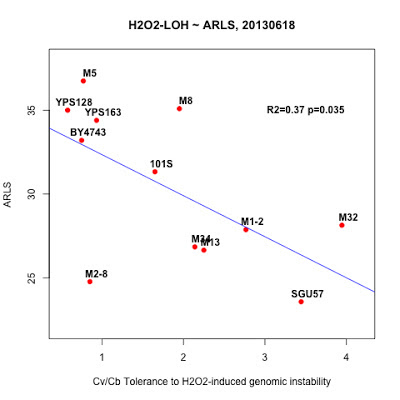
*** H2O2 induced LOH ~ ARLS: Tradeoff between robustness and replicative lifespan

------
2013Dec5 comments
M2-8 has a dilution bias and was not fitted correctly in this plot.
M32 is a tricky strain that we repeated at least 5 times.
----------

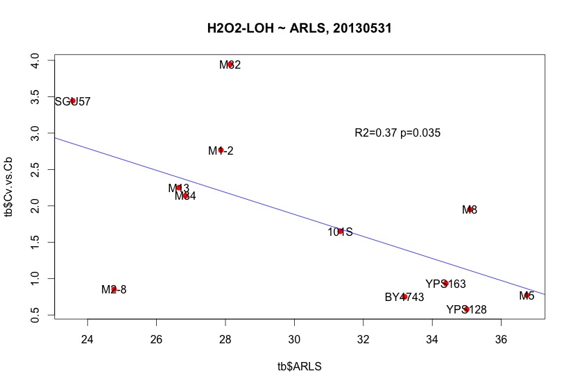Large Cv/Cb indicate better survival ship beyond H2O2-induced LOH. The negative correlation indicates a trade off
between Cv/Cb and RLS. 

plot( tb$Cv.vs.Cb ~ tb$ARLS, pch=19, col="red", main="H2O2-LOH ~ ARLS, 20130531" )
 text( tb$ARLS, tb$Cv.vs.Cb, tb$strain)
 m = lm(tb$Cv.vs.Cb ~ tb$ARLS )
 abline( m, col="blue")
 summary(m)
 text(33, 3, "R2=0.37 p=0.035")

Small L0 indicates better asymmetry. Large Cv/Cb indicates better tolerance to H2O2 or
more sensitive to H2O2. So, this negative correlation actually indicates a positive relationship
between Cv/Cb and mitotic asymmetry. 

 plot( tb$Cv.vs.Cb ~ tb$L0.all , pch=19, col="red", main="H2O2-LOH ~ mitotic asymmetry, 20130531" )
 text( tb$L0.all, tb$Cv.vs.Cb, tb$strain)
 m = lm(tb$Cv.vs.Cb ~ tb$L0.all )
 abline( m, col="blue")
 summary(m)
 text(0.2, 3.5, "R2=0.42 p=0.031")

Updated on 2013 June 18. I switched x-y axis for more clear presentation.

Updated on 2013 June 18.

Conclusions:  
 Cv/Cb ~(-)~ ARLS
 Tc/Tg ~(-)~ ARLS
  G       ~(-)~ ARLS
Morphological robustness ~(-)~ RLS ?
Growth fitness ~(+)~ RLS ?


Reference:
_2013May31-H2O2LOH.R
_2013June18-H2O2LOH.R

LOH and robustness, Tc/Tg ~ ln(R) + G, Strehler-Mildvan correlation in wild yeast

"_2013May29,R0-G-TcTg.regression.by.mean.R" in  /Users/hongqin/projects/LOH_H2O2_2012-master/analysis. The ARLS data is from Qin06EXG. 


 rm( list = ls() );
 tb = read.table("summary.new.by.strain.csv", header=T, sep="\t");
 tb.old = tb;
 labels = names( tb.old );
 #tb = tb.old[c(1:11), c(1:5,8, 10, 12, 14, 16, 18, 20, 22)]

 tb = tb.old[c(1:11), c("strain","ARLS","R0","G","CLS","Tc", "Tg","Tmmax","Tbmax", "Td", "Tdmax","TLmax","Lmax", 
 "b.max", "b.min", "strains", "L0.all", "L0.small" , "Pbt0","Pb0.5t0", "Pbt0.b") ];

 tb$CLS.vs.Tc = tb$CLS / tb$Tc; 
 tb$Tg.vs.Tc = tb$Tg / tb$Tc;
 tb$Tc.vs.Tg = tb$Tc / tb$Tg

> summary( lm( tb$Tc.vs.Tg ~ log(tb$R0) + tb$G  ) )

Call:

lm(formula = tb$Tc.vs.Tg ~ log(tb$R0) + tb$G)

Residuals:

     Min       1Q   Median       3Q      Max 

-0.16512 -0.04416 -0.01631  0.03805  0.22175 

Coefficients:

            Estimate Std. Error t value Pr(>|t|)   

(Intercept)  1.58691    0.31955   4.966  0.00110 **

log(tb$R0)   0.22037    0.06505   3.388  0.00953 **

tb$G         4.68078    1.68987   2.770  0.02430 * 

---

Signif. codes:  0 ‘***’ 0.001 ‘**’ 0.01 ‘*’ 0.05 ‘.’ 0.1 ‘ ’ 1 

Residual standard error: 0.1101 on 8 degrees of freedom

Multiple R-squared: 0.5991, Adjusted R-squared: 0.4989 

F-statistic: 5.977 on 2 and 8 DF,  p-value: 0.02584 

require(scatterplot3d);
s3d <- scatterplot3d( log(tb$R0), tb$G, tb$Tc.vs.Tg,  type='h',color="red", pch=16,
                      main="Correlations among Tc/Tg, log(R0), and G", 
                      angle=40, scale.y=0.7
);
my.lm <- lm( tb$Tc.vs.Tg ~ log(tb$R0) + tb$G);
s3d$plane3d( my.lm, lty.box="solid");

text(s3d$xyz.convert( tb$Tc.vs.Tg, log(tb$R0), tb$G), labels=tb$strain, pos=1)

> model = lm(log(tb$R0) ~ tb$G )
> summary( model ) #p=0.02, strehler-mildvan correlation!

Call:
lm(formula = log(tb$R0) ~ tb$G)

Residuals:
     Min       1Q   Median       3Q      Max 
-0.86676 -0.45345 -0.04328  0.40139  0.80255 

Coefficients:
            Estimate Std. Error t value Pr(>|t|)    
(Intercept)  -4.2158     0.8407  -5.015 0.000724 ***
tb$G        -17.2886     6.4637  -2.675 0.025425 *  
---
Signif. codes:  0 ‘***’ 0.001 ‘**’ 0.01 ‘*’ 0.05 ‘.’ 0.1 ‘ ’ 1 

Residual standard error: 0.5641 on 9 degrees of freedom
Multiple R-squared: 0.4429, Adjusted R-squared: 0.381 

F-statistic: 7.154 on 1 and 9 DF,  p-value: 0.02543 
> plot( log(tb$R0) ~ tb$G, pch=19, ylim=c(-8, -5), xlim=c(0.07, 0.17) )
> title("p=0.025, Strehler-Mildvan, natural isoaltes")
> text( tb$G*1.01, log(tb$R0)*1.02, tb$strain)
> abline(model, col='red')

> tb

   strain     ARLS        R0         G       CLS       Tc        Tg     Tmmax     Tbmax        Td     Tdmax     TLmax      Lmax      b.max

1    101S 31.32761 0.0012098 0.1421899  3.393531 4.580000  5.686667  5.483333  5.633333  4.786667  4.786667  6.653333 2.4900000 0.04333333

2    M1-2 27.86968 0.0024437 0.1283620 10.370586 6.273333  6.930000  7.316667  6.833333  6.930000  6.930000  7.653333 0.7066667 0.04000000

3     M13 26.65020 0.0029551 0.1252717 16.273320 8.010000 11.053333  9.433333 11.083333  9.246667  9.246667  9.666667 0.6533333 0.13666667

4     M14 36.58444 0.0018812 0.0949553  7.212224 3.960000  7.043333  4.900000  7.016667  5.840000  5.840000  9.500000 1.2000000 0.16333333

5    M2-8 24.77079 0.0041838 0.1193465  4.124016 4.122500  4.507500  5.100000  4.487500  5.870000  5.870000  7.020000 3.3450000 0.03425000

6     M32 28.13750 0.0017568 0.1417765  6.422428 7.963333  7.413333  9.733333  7.350000  8.206667  8.206667  7.626667 0.5966667 0.03000000

7     M34 26.84275 0.0012919 0.1629953  5.167521 6.732500  8.212500  8.325000  8.300000  8.382500  8.382500  7.552500 0.7925000 0.22250000

8      M5 36.74289 0.0040310 0.0681621  4.934625 5.920000  7.816667  7.050000  7.833333  6.546667  6.546667  6.906667 1.8400000 0.24333333

9      M8 35.09139 0.0003775 0.1619232 10.492830 6.783333 11.466667  8.216667 11.516667  6.026667  6.026667  6.873333 1.2400000 0.16666667

10 YPS128 34.99853 0.0011183 0.1209893  3.309616 8.630000 12.873333 10.750000 12.450000 11.420000 11.420000 11.766667 1.7333333 0.20666667

11 YPS163 34.39308 0.0008251 0.1350900  4.184502 5.246667  8.310000  6.850000  8.283333  7.140000  7.140000  5.246667 1.3266667 0.16333333

        b.min strains     L0.all   L0.small       Pbt0    Pb0.5t0     Pbt0.b CLS.vs.Tc  Tg.vs.Tc  Tc.vs.Tg

1  0.00000000    101S 0.15957447 0.09523810 0.00280093 0.00026676 0.00277755 0.7409457 1.2416303 0.8053927

2  0.00000000    M1-2 0.06164384 0.03571429 0.00183932 0.00006569 0.00189366 1.6531221 1.1046759 0.9052429

3  0.00000000     M13 0.09345794 0.12500000 0.00197697 0.00024712 0.00214845 2.0316255 1.3799417 0.7246683

4  0.00333333     M14 0.11224490 0.10975610 0.00699718 0.00076798 0.00660394 1.8212687 1.7786195 0.5622338

5  0.00000000    M2-8 0.14859438 0.16363636 0.00366569 0.00059984 0.00390693 1.0003677 1.0933899 0.9145868

6  0.01000000     M32 0.10962567 0.13440860 0.01235470 0.00166058 0.01252386 0.8065000 0.9309334 1.0741906

7  0.00250000     M34 0.17134831 0.16176471 0.00727065 0.00117614 0.00688487 0.7675486 1.2198292 0.8197869

8  0.00000000      M5 0.17187500 0.17948718 0.00200535 0.00035993 0.00206424 0.8335515 1.3203829 0.7573561

9  0.00000000      M8 0.05810398 0.07471264 0.00637153 0.00047603 0.00633754 1.5468545 1.6904177 0.5915698

10 0.01333333  YPS128 0.18353175 0.09166667 0.01086710 0.00099615 0.01106367 0.3835013 1.4916956 0.6703780

11 0.00666667  YPS163 0.25268817 0.09032258 0.00712283 0.00064335 0.00824009 0.7975545 1.5838628 0.6313678